Project 3 Part 1: PathTracer

Overview

In this project, we created the infrastructure necessary to produce basic path tracing images with diffuse shading. This included:

• Calculating ray-scene intersections (between spheres and triangles)
• Generating the Bounding Volume Hierarchy acceleration structure
• Implementing the Diffuse BSDF
• Creating algorithms for direct, indirect, and global illumination using Monte Carlo estimation and Russian Roulette ray termination
• Adaptive sampling rates for further rendering speed-up

Part 1: Ray Generation and Scene Intersection

In this part, we implemented ray generation from the camera perspective, as well as ray-triangle intersections and ray-sphere intersections.

The ray generation pipeline is as follows:

1. We determine the $(x, y)$ coordinates in screen space of a particular pixel we would like to cast a ray into.
2. Using Monte Carlo sampling, we randomly generate a ray at uniform random through the region bounded by $(x, y)$ and $(x+1), (y+1)$.
3. We pass the normalized (between 0 and 1) screen coordinates into the Camera::generate_ray() function.
4. In generate_ray(), we transform the provided screen space coordinates into world space coordinates by first transforming into camera space using the FOV values, then into world space by rotating by the c2w transform.
5. If applicable, we check for intersections with objects. If an intersection is detected, we terminate the ray at the intersection (set max_t to the intersection time).

Our triangle intersection algorithm worked in three parts, based on the Möller-Trumbore algorithm:

1. Determine when the ray will intersect with the plane the triangle is on, or if it will not intersect at all, by calculating the plane normal via a cross product of two edges. Terminate immediately if the ray is parallel to the plane.
2. Check that point where the ray intersects the plane is within the triangle and the t value is between min_t and max_t using barycentric coordinates. $\alpha, \beta$ can be calculated using a weighted dot product of orthogonal vectors based on the intersection point and triangle edges.
3. Calculate the normal vector using barycentric coordinates, weighting the vertex normals $n1, n2, n3$ by $\alpha, \beta, \gamma$ respectively.

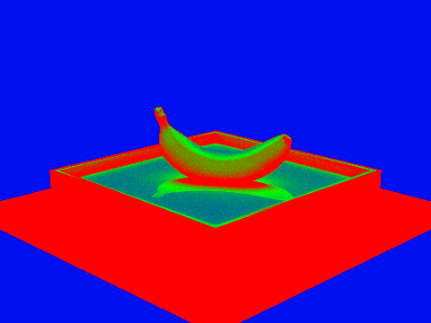
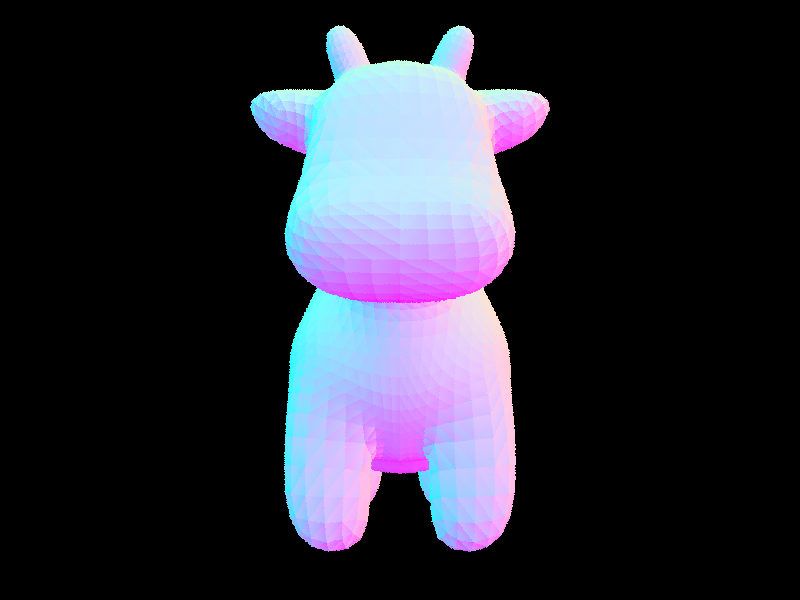
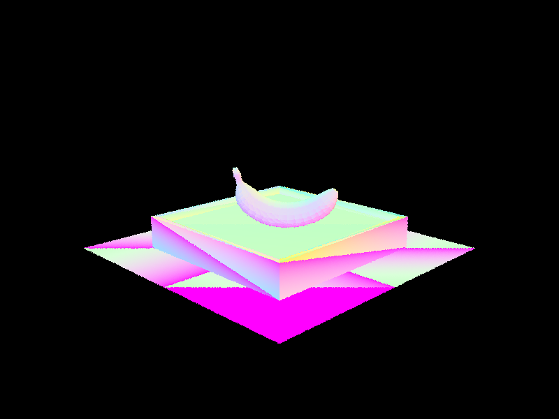
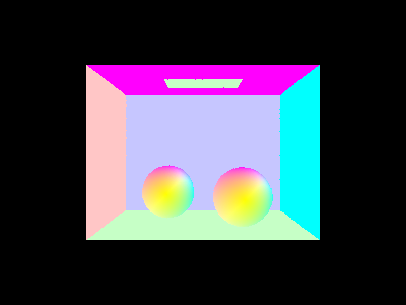
Demo Images

Cow: Banana: Sphere:

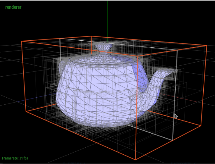
Part 2: Bounding Volume Hierarchy

Creating the BVH

In this part, we implemented the BVH acceleration structure to dramatically increase the performance of path tracing.

The algorithm for generating the bounding volume hierarchy is as follows:

1. First, check if the current node is a leaf node. If so, simply set its start and end values, then return it. Otherwise, it’s an inner node, so we should continue with the algorithm to split.
2. Find the centroid of the current bounding box.
3. Create six lists corresponding to the objects to the left and right of each axis of the centroid.
4. Iterate over all objects in the current box, and add them to three of the six lists depending on its position. (For example, if the centroid is $(1,1,1)$ and an object is at $(0,0,2)$, it should be added to x_left, y_left, and z_right).
5. Select the axis with the most even split (greatest size of the smallest list out of the left and right).
6. Create a left and right node with the left and right lists of the selected axis, and pass these into two recursive calls.

Here is a screenshot of the teapot mesh demonstrating the appearance of the BVHNodes:

BVH Demos

Demos were rendered on an Ubuntu 22.04 virtual machine with 6 Ryzen 7 3700x cores, 16GB RAM, and a GTX 1080.

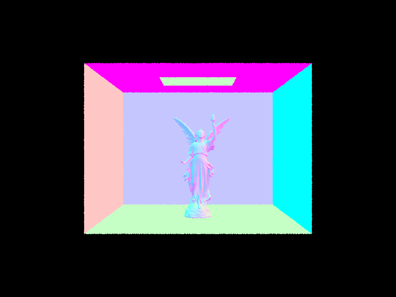
Lucy

• 133,796 primitives
• Rendering Time: 0.0767s
• Average speed: 5.6005 million rays per second
• Intersection tests per ray: 1.784651

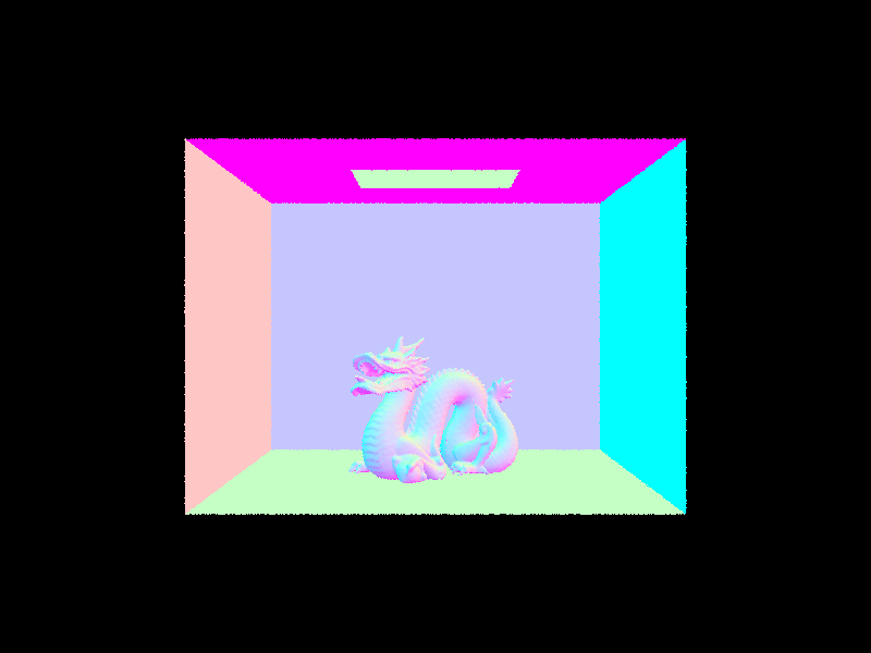
Dragon

• 110,012 primitives
• Rendering Time: 0.0930s
• Average speed: 4.9570 million rays per second
• Intersection tests per ray: 3.377663

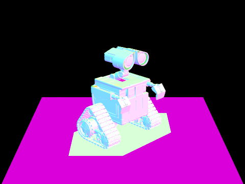
Wall-E

• 240,326 primitives

Part 3: Direct Illumination

We wrote two direct lighting functions: one using uniform hemisphere sampling and the other using importance sampling. For uniform hemisphere sampling, we took num_sample sample rays eminating from the hit point and uniformly chosen from the hemisphere around the hit point. The algorithm works as follows for each sample ray:

1. Determine if the ray will intersect with another object in the scene using intersect and save the intersection in light_isect.
2. If there is an intersecion we calculate the contribution to our object’s brightness at the hit point using the reflection equation. The values used are in the next 3 steps
3. $f_r$ is determined using bsdf->f of the object.
4. $L$ is determined by the by the emission of the intersected light. If the object the sample ray intersects with is not a light, then it contributes no brightness.
5. The angle is determined using cos_theta of the sample ray’s direction
6. We add the contribution of this sample to L_out Once we calculate the contribution of all of the samples, we normalize by the number of samples and return that result as the brightness of the object at the hit point.

For importance sampling, we iterated through all of the light sources in the scene, and estimated their contribution to the lighting of the object. The algorithm works as follows for each light source:

1. If it is a point light we take only one sample, otherwise we take ns_area_light samples
2. For each sample we determine whether the light is behind the object and if there is anything blocking the light in the following two steps
3. We trace a ray from the light to the hit point, if the distance is positive then we know that the light is behind the object
4. We check if there is an object between the object and the light using intersect with the max_t set to the distance from the light to the object. If we do not intersect anything, then we can add the light’s contribution to the brightness of the hit point, normalized by the pdf for that light and the number of samples. Once we calculate the contribution from all of the light sources we return that result as the brightness of the object at the hit point.

Demos: Hemispheric vs Importance Sampling

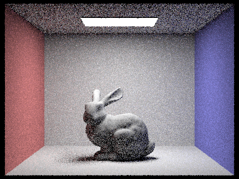
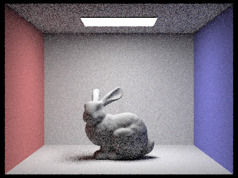
Hemispheric sampling takes much longer to resolve compared to Importance sampling given the same number of samples. Additionally, the image generated by hempispheric sampling is noisier and darker. The difference is due to hemispheric sampling simply taking random sample rays eminating from the hit point, most of which will not intersect with a light source. This means that hemispheric sampling will require a lot of samples for each point to have a good approximation of how much light shines onto each point. In contrast, importance sampling samples over the light sources and so is guaranteed to sample rays between the light sources and the point, which allows it to converge much faster. As a result, our importance sampling image is clear and rendered faster while the hemispheric sampling image is still noisy and rendered slower. More importantly, for the second image with only a point light, hemispheric sampling resulted in a completely black image whereas importance sampling rendered the correct image of a banana. Hemisphereic sampling failed in this case, because the probability of a randomly generated ray from any point exactly intersecting the point light is zero, and so none of the points had sample rays that contributed brightness to that point. In contrast, importance sampling generated samples using the point and so could accuractly render how that point light would light up the entire scene.

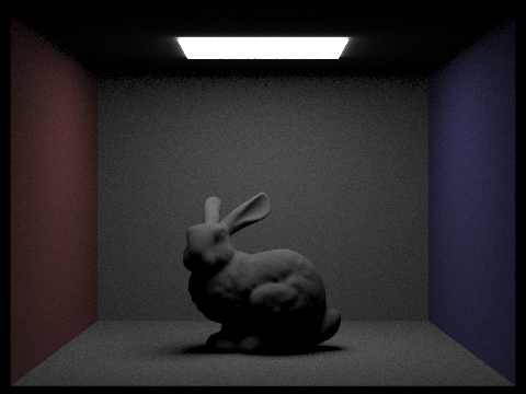
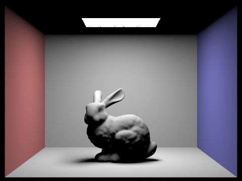
Bunny wih direct illumination and hemispheric sampling

./pathtracer -t 8 -s 64 -l 32 -m 6 -H -f CBbunny_H_64_32.png -r 480 360 ../dae/sky/CBbunny.dae

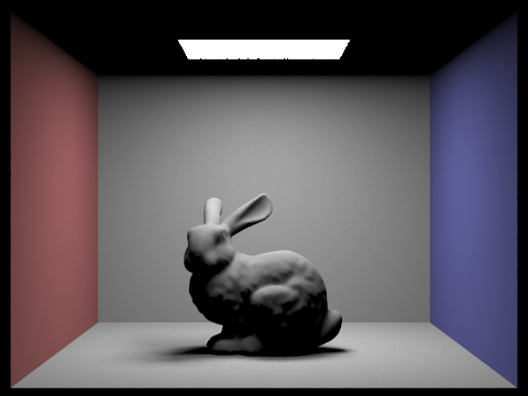
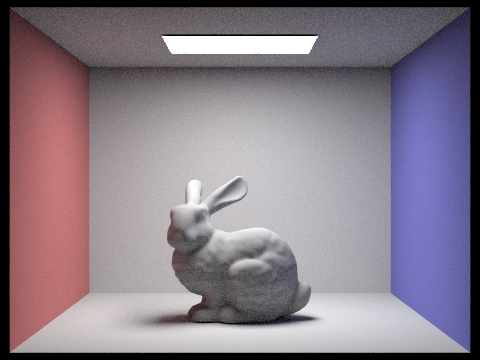
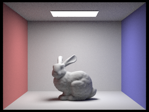
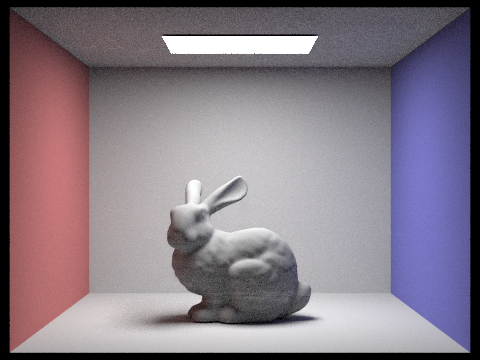
Bunny with direct illumination and importance sampling

./pathtracer -t 8 -s 64 -l 32 -m 6 -f CBbunny_H_64_32.png -r 480 360 ../dae/sky/CBbunny.dae

Banana with direct illumination and hemispheric sampling

./pathtracer -t 8 -s 64 -l 32 -m 6 -H -f banana_H.png -r 480 360 ../dae/keenan/banana.dae

the banana appears black because hemispheric sampling does not render point lights

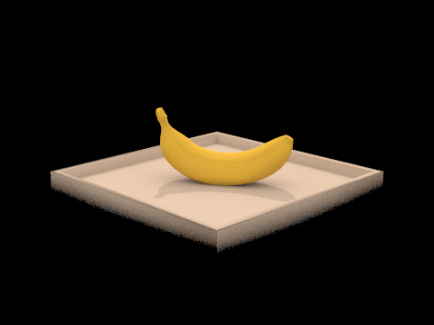
Banana with direct illumination and importance sampling

./pathtracer -t 8 -s 64 -l 32 -m 6 -f banana_I.png -r 480 360 ../dae/keenan/banana.dae

Demos: Noise Levels

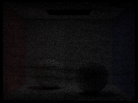
Noise levels in soft shadows using light sampling:

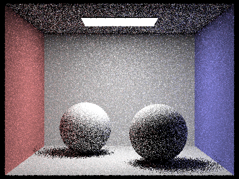
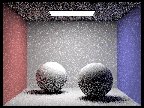
Light rays: 1

./pathtracer -t 8 -s 1 -l 1 -m 6 -f spheres_l1.png -r 480 360 ../dae/sky/CBspheres_lambertian.dae

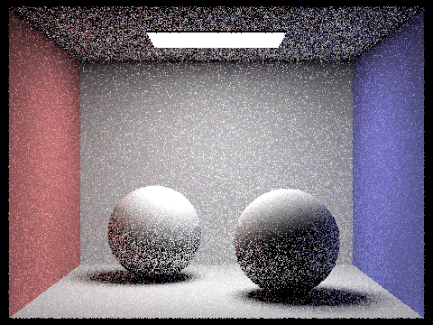
Light rays: 4

./pathtracer -t 8 -s 1 -l 4 -m 6 -f spheres_l4.png -r 480 360 ../dae/sky/CBspheres_lambertian.dae

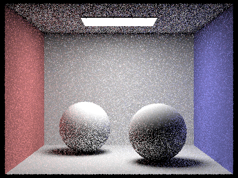
Light rays: 16

./pathtracer -t 8 -s 1 -l 16 -m 6 -f spheres_l16.png -r 480 360 ../dae/sky/CBspheres_lambertian.dae

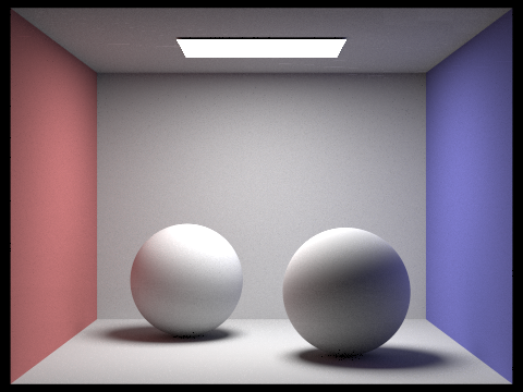
Light rays: 64

./pathtracer -t 8 -s 1 -l 64 -m 6 -f spheres_l64.png -r 480 360 ../dae/sky/CBspheres_lambertian.dae

Part 4: Global Illumination

We implemented indirect lighting via a monte carlo estimator with russian roulette for random termination. Our at_least_one_bouce_radiance function works recursively where we determine how much light is emitted from an object by calling at_least_one_bounce_radiance on it. The algorithm works as follows:

1. Base Case: When there are no further bounces, we return the one_bounce_radiance of the object at the hit point according to the algorithms from part 3.
2. Recursive Case: We randomly sample a ray eminating from the hit point and if it hits an object, we use the reflectance equation to determine the contribution of that intersected object to our hit point. The light of the intersected object is calculated recursively using at_least_one_bounce_radiance. We keep count of each recursion and terminate at the base case when there are no further bounces. Additionally, we have a chance to randomly terminate based on our Russian Roulette constant. Finally, if the sampled ray has no intersection, the recursion terminates.

Demos of Global Illumination

Global Illumination

./pathtracer -t 8 -s 1024 -l 16 -m 5 -r 480 360 -f spheres_global.png ../dae/sky/CBspheres_lambertian.dae

Only Direct Illumiation (run direct illumination)

./pathtracer -t 8 -s 1024 -l 16 -r 480 360 -f spheres_dir_only.png ../dae/sky/CBspheres_lambertian.dae

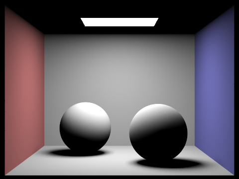
Only Indirect Illumination (edited at_least_one_bounce_radiance())

./pathtracer -t 8 -s 1024 -l 16 -m 5 -r 480 360 -f spheres_indir_only.png ../dae/sky/CBspheres_lambertian.dae

Comparison of max_ray_depth

Max Ray Depth: 0

./pathtracer -t 8 -s 64 -l 32 -m 0 -f CBbunny_m0.png -r 480 360 ../dae/sky/CBbunny.dae

Max Ray Depth: 1

./pathtracer -t 8 -s 64 -l 32 -m 1 -f CBbunny_m1.png -r 480 360 ../dae/sky/CBbunny.dae

Max Ray Depth: 2

./pathtracer -t 8 -s 64 -l 32 -m 2 -f CBbunny_m2.png -r 480 360 ../dae/sky/CBbunny.dae

Max Ray Depth: 3

./pathtracer -t 8 -s 64 -l 32 -m 3 -f CBbunny_m3.png -r 480 360 ../dae/sky/CBbunny.dae

Max Ray Depth: 100

./pathtracer -t 8 -s 64 -l 32 -m 100 -f CBbunny_m100.png -r 480 360 ../dae/sky/CBbunny.dae

Comparison of various sample-per-pixel

sample-per-pixel: 1

./pathtracer -t 8 -s 1 -l 4 -m 5 -f CBbunny_s1.png -r 480 360 ../dae/sky/CBbunny.dae

sample-per-pixel: 2

./pathtracer -t 8 -s 2 -l 4 -m 5 -f CBbunny_s2.png -r 480 360 ../dae/sky/CBbunny.dae

sample-per-pixel: 4

./pathtracer -t 8 -s 4 -l 4 -m 5 -f CBbunny_s4.png -r 480 360 ../dae/sky/CBbunny.dae

sample-per-pixel: 8

./pathtracer -t 8 -s 8 -l 4 -m 5 -f CBbunny_s8.png -r 480 360 ../dae/sky/CBbunny.dae

sample-per-pixel: 16

./pathtracer -t 8 -s 16 -l 4 -m 5 -f CBbunny_s16.png -r 480 360 ../dae/sky/CBbunny.dae

sample-per-pixel: 64

./pathtracer -t 8 -s 64 -l 4 -m 5 -f CBbunny_s64.png -r 480 360 ../dae/sky/CBbunny.dae

sample-per-pixel: 1024

./pathtracer -t 8 -s 1024 -l 4 -m 5 -f CBbunny_s1024 -r 480 360 ../dae/sky/CBbunny.dae

Part 5: Adaptive Sampling

Adaptive Sampling aims to speed up rendering by sampling pixels at different rates based on how fast they converge to their true value. The different rates are chosen such that the pixels that converge quickly have fewer samples taken compared to the pixels that converge slowly. Our function implements adaptive sampling by checking whether a pixel has converged, and then stops taking new samples if it has converged. This check uses the following equations: (as per the spec):

1. $I = 1.96 * \frac{\sigma}{\sqrt{n}}$ where $n$ is the number of samples we’ve already traced, and $\sigma$ is the standard deviation of the sample values
2. $I <= maxTolerance * \mu$ where $\mu$ is the average value of the samples taken so far

$I$ is a value based on the sample’s standard deviation, which gets smaller as the pixel’s value converges. The second equation is our check that $I$ is sufficiently small for us to conclude that the pixel has converged and so we stop taking new samples We calculate $\mu$ and $\sigma$ for the set of samples at a pixel using a rolling sum of illumination (given in the illum() function) and illumination squared. The mean and variance of the samples so far are then calculated using those values. Finally, we only check if a pixel has converged every samplesPerBatch samples so as to reduce the number of times we did the calculation to check. This gave a balance between terminating the loop early without adding too much additional computation in each loop.

Demos of adaptive sampling

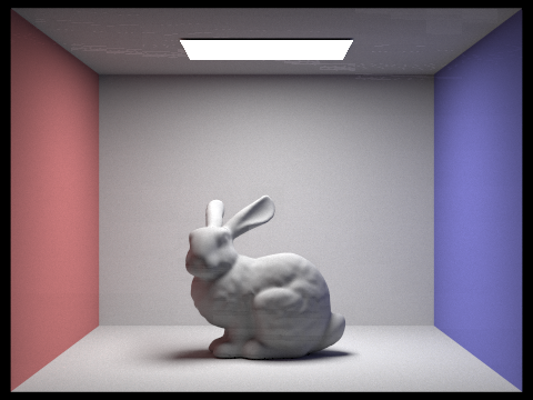
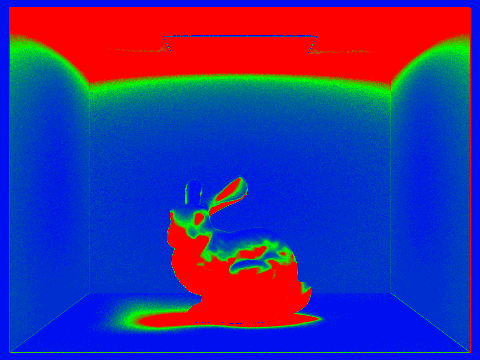
Bunny

./pathtracer -t 8 -s 2048 -a 64 0.05 -l 1 -m 6 -r 480 360 -f bunny_as.png ../dae/sky/CBbunny.dae

Produced Image: Rate Heatmap:

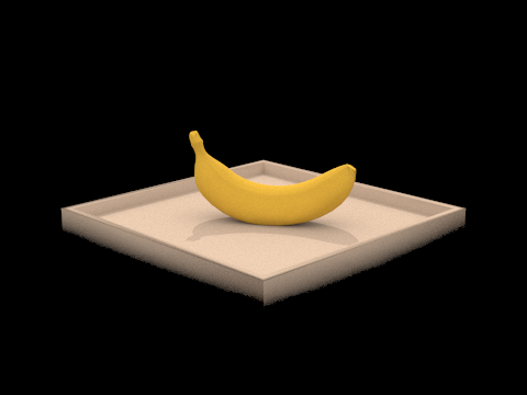
Banana

./pathtracer -t 8 -s 2048 -a 64 0.05 -l 1 -m 6 -r 480 360 -f banana_as.png ../dae/keenan/banana.dae

Produced Image:

Rate Heatmap: