Project 2: MeshEdit

Overview

In this project, we implemented several common structures and algorithms used to rasterize 2D curves and 3D meshes based on the Half-Edge data structure.

Specifically, we allow input as either Bezier curves/surfaces (.bez, .bzc) or Digital Asset Exchange (.dae) files, and render them onto the screen. We also implemented the de Castellau subdivision algorithm for upsampling 2D curves, and the Loop subdivision algorithm to upsample 3D meshes. In the process, we also had to implement edge flipping and edge splitting in 3D meshes.

Section I: Bezier Curves and Surfaces

Part 1: Bezier Curves

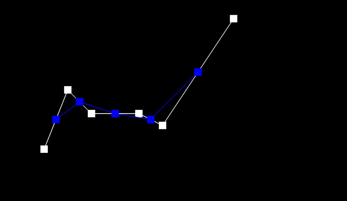
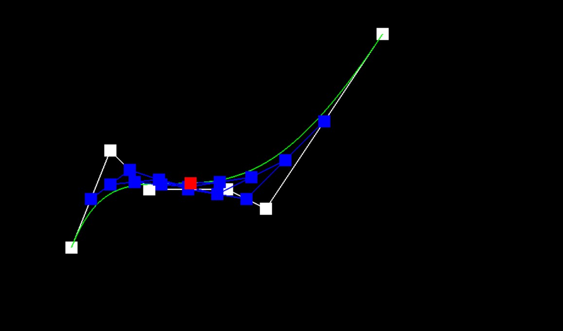
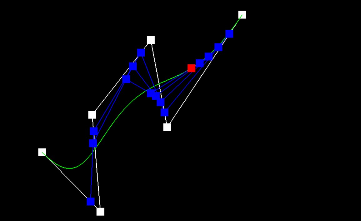
The de Casteljau algorithm evaluates Bezier curves using multiple steps of linear interpolation. For a given $t$ such that $0 \le t \le 1$, on each step, the algorithm finds a point that splits the neighboring two points into $t$ and $1-t$ fractions. The next steps use the points found in the previous step, each time decreasing the number of points by one until there is only one point. That final point must be on the Bezier curve, so by sampling regular intervals of $t$ along the curve we can approximate the curve when rasterizing.

In the project we evaluate one step at a time in the evaluateStep function using a for loop up to the second to last point provided, each time evaluating what the point for the next step should be using linear interpolation and adding it to a result vector. Once finished, we return the result vector. As the base case, if the input vector contains only one point, then we return that point.

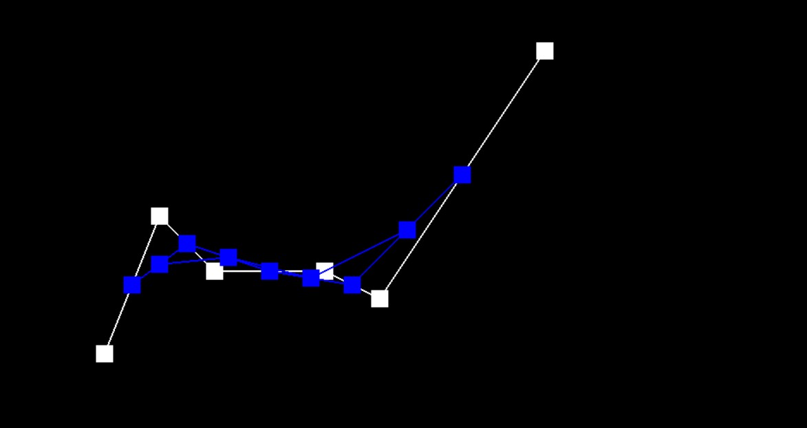
Each Step of Evaluation:

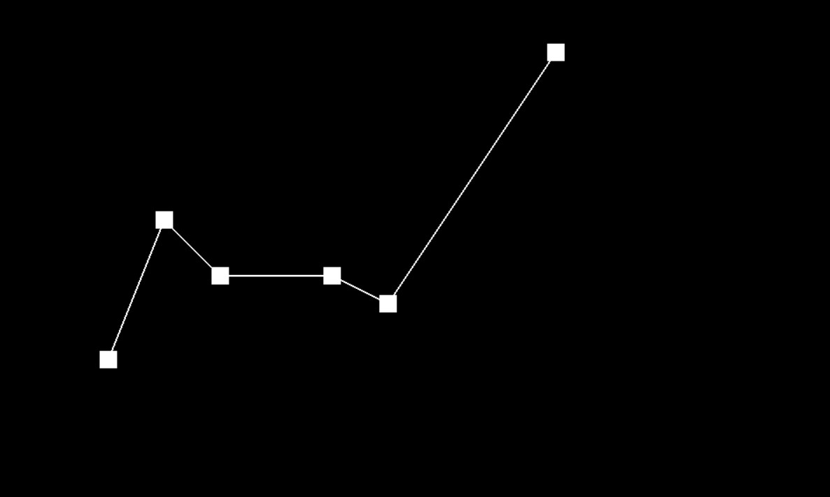
For this part, we created a custom 6-control-point Bezier curve with the following source code:

6
0.200 0.350
0.300 0.600
0.400 0.500
0.600 0.500
0.700 0.450
1.000 0.900

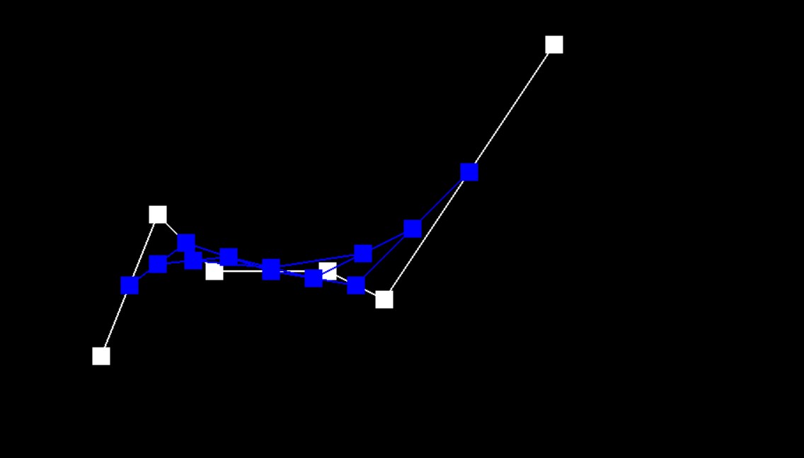
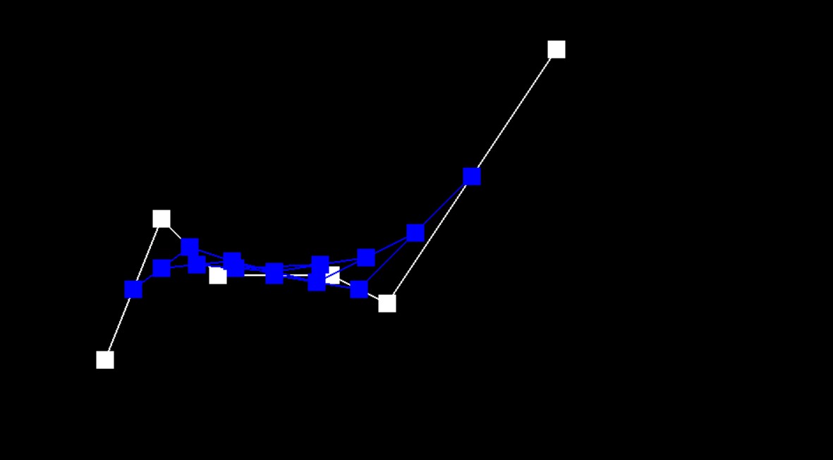
Step 0 Step 1 Step 2 Step 3 Step 4 Step 5 (final step)

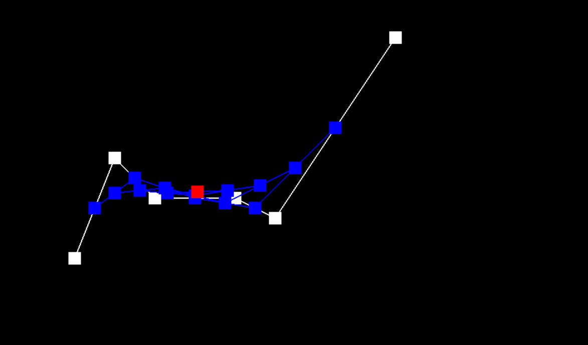
Completed Bezier Curve

Slightly Different Bezier Curve

Part 2: Bezier Surfaces

The de Casteljau algorithm extends to Bezier surfaces via a two step process: the first step is to evaluate the final point for each row of points along one axis, the second step uses those points to evaluate the final point along the other axis. The $t$ used for both axes can be different (inputted as $u$ and $v$, respectively).

In the project, the evaluate function performs the two steps explained above on the $N$-by-$N$ set of control points by calling evaluate1D for each row, then for the vector created by the points evaluated from each row. evaluate1D evaluates the final point by calling evaluateStep on the given set of points until there is only the final point left. Finally, evaluateStep performs the same operation as evaluate in part 1, except that the $t$ value is provided to the function instead of being a parameter of BezierCurve.

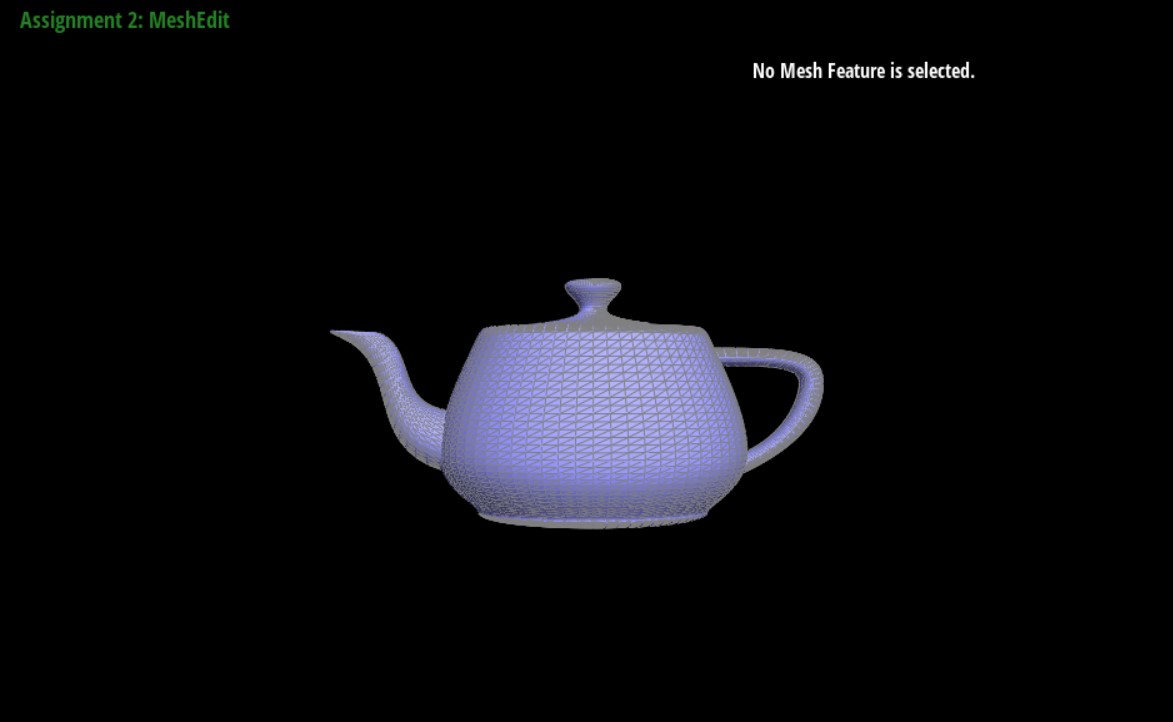
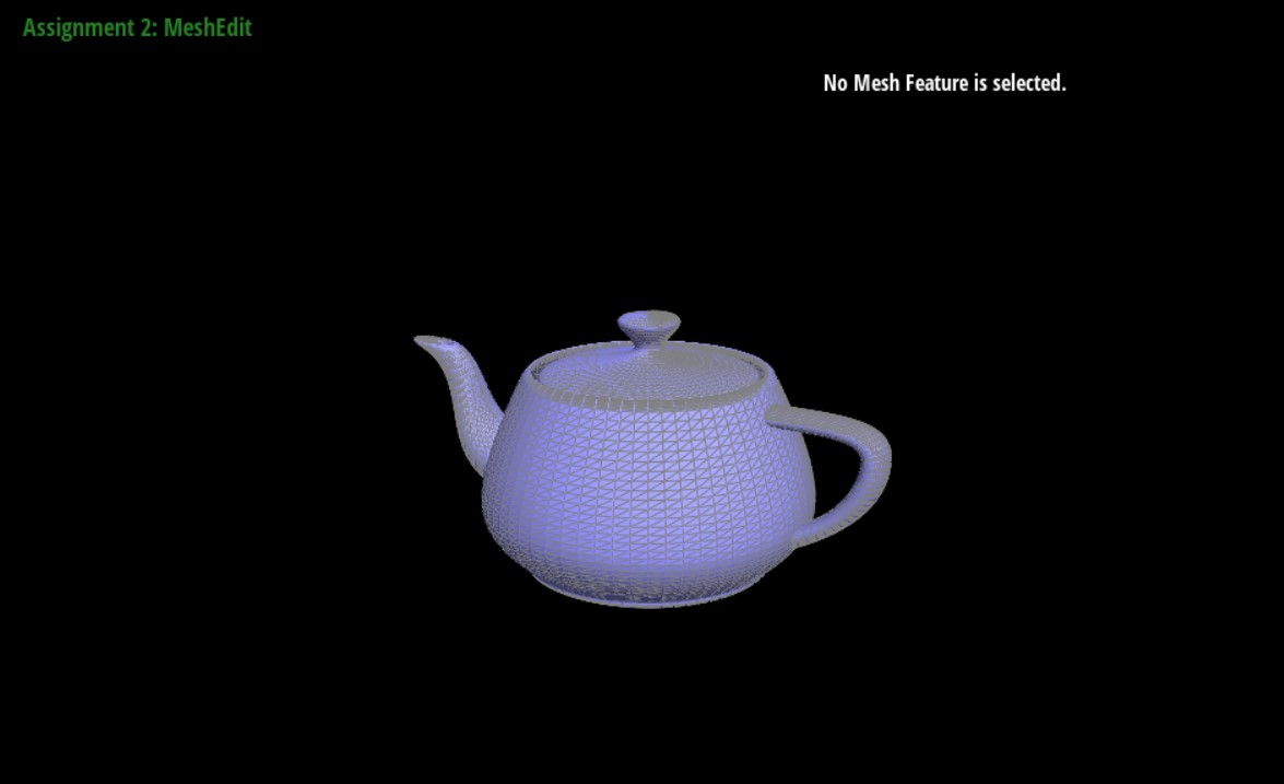
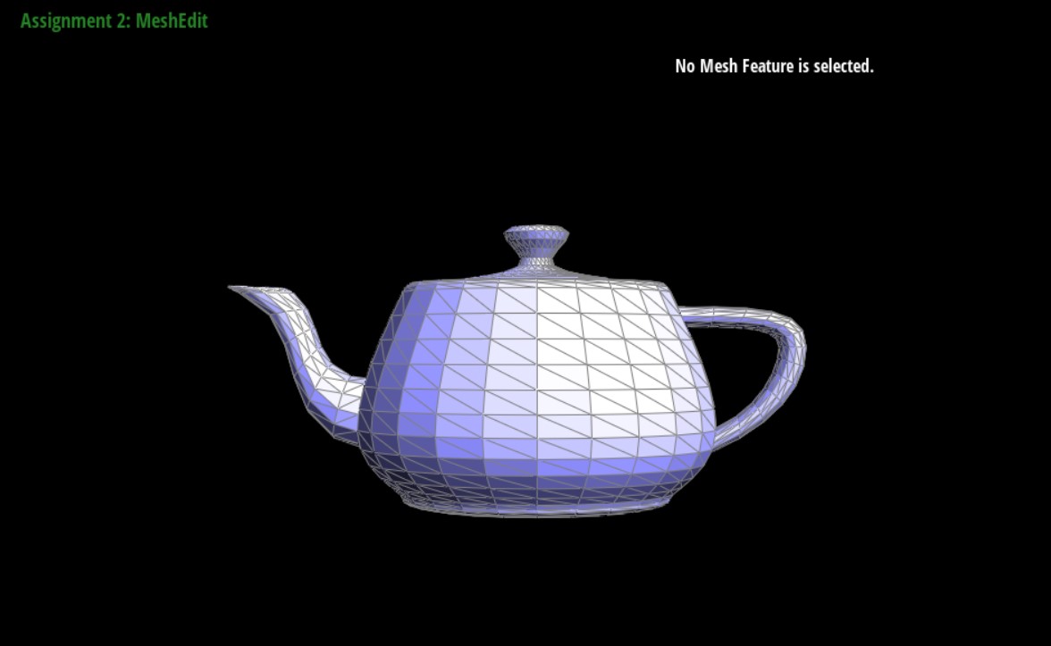
Images of teapot.bez as rendered with our Bezier Surfaces functions

Section II: Triangle Meshes and Half-Edge Data Structure

Part 3: Area-Weighted Vertex Normals

To calculate the area-weighted vertex normals we calculated the area-weighted average of the normals of all neighboring triangles to the vertex, then normalized that result.

The algorithm for doing so involves iterating through all neighboring triangles in a loop, which can be done by going from the current half edge’s twin()->next().

For each triangle, we do the following:

1. Find the three vertices $A$, $B$, and $C$ using basic half-edge traversal (h->next() then h->next()->next()).
2. Calculate the triangle’s area using the formula $\frac{1}{2} | \text{len one side} * \text{len another side} |$. Specifically, this can be written in terms of vertex locations: $\frac{1}{2} | (A - B) \times (C - B) |$.
3. Get the unit vector for the face normal, and multiply it by area found in the previous calculation. Add it to our running total.

Finally, we normalized the running total and returned that as the current vertex’s normal vector.

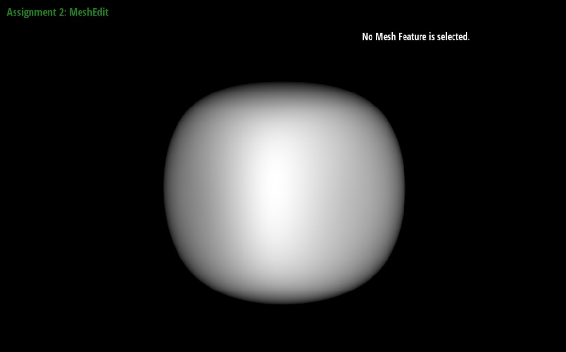
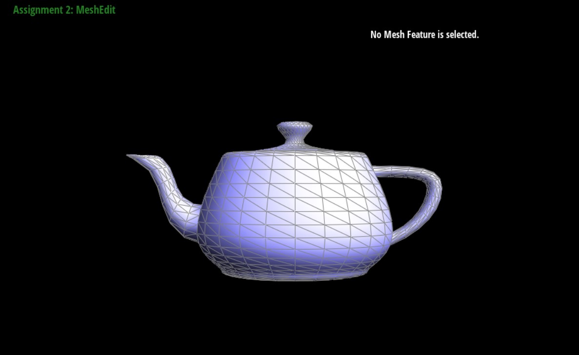
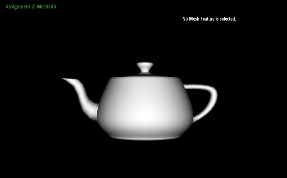
Images of teapot.dae with and without Phong shading

Without Phong shading

With Phong shading

Without the wire framing, to see the shading more clearly

Part 4: Edge Flip

Here is the diagram and table we made to guide our implementation:

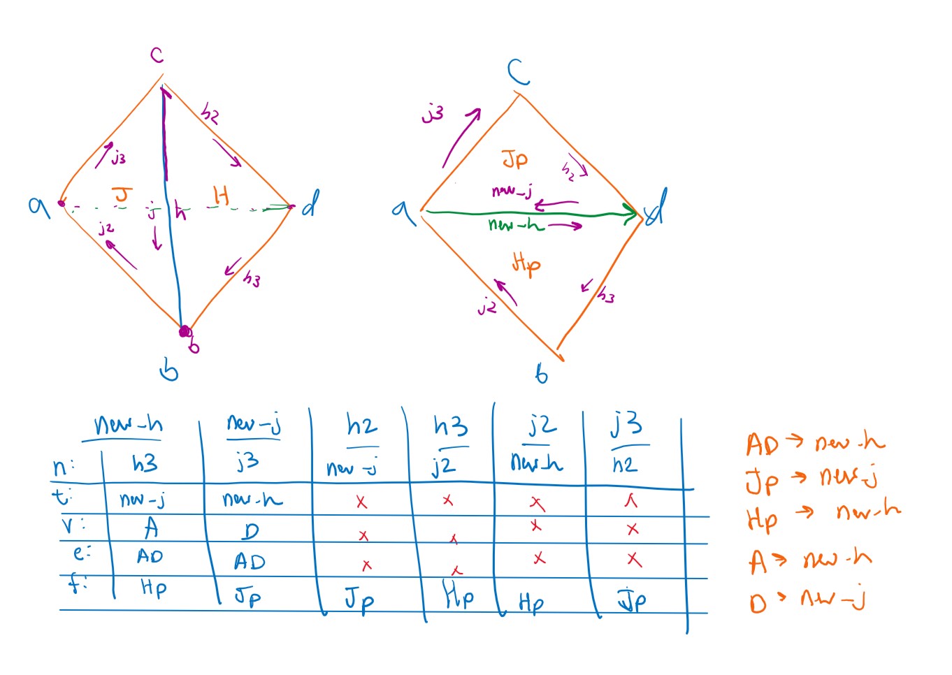
We implemented the changes listed in the table above. Notably, we do the following:

1. Find all of the components in the diagram using half-edge traversal, and assign them to the naming scheme shown in the diagram.
2. Reassign the pointers of those components according to our table above. (Each column in the table corresponds to one half-edge, and the faces/vertices/edges are displayed on the right of the table.)

Images before/after edge flips

Before Edge Flips

After Flipping the Lower Edge

Debugging journey: At first we had created new mesh elements for the new components, but quickly realized that the spec prohibited adding or deleting mesh elements. So we changed our implementation to reuse the elements we were deleting into the new elements by reassigning their pointers.

We realized the points B and C (in diagram) might have different halfedges than expected since the halfedge of a vertex can be any of the emanating halfedges, so we explicitly redefined their halfedges.

We also found that using cube.dae was far easier for testing than teapot, since it is easier to visualize what should happen and it is faster to load.

Part 5: Edge Split

Here is the diagram and table we made to guide our implementation:

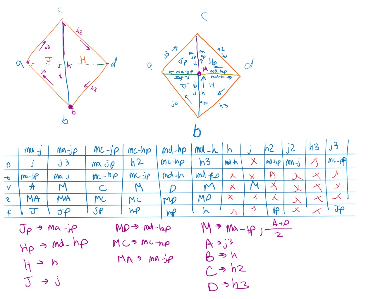
We implemented the changes listed in the table in three steps:

1. Find all the pre-existing components in the diagram and named them according to our diagram
2. Instantiate the new components (three edges MA, MC, MD; six half-edges, two for each of the new edge; one vertex M)
3. Assign all the pointers of the old and new components according to our table.

Images before/after Edge splits and flips

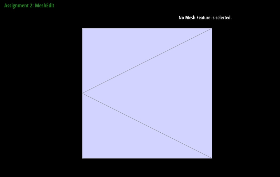
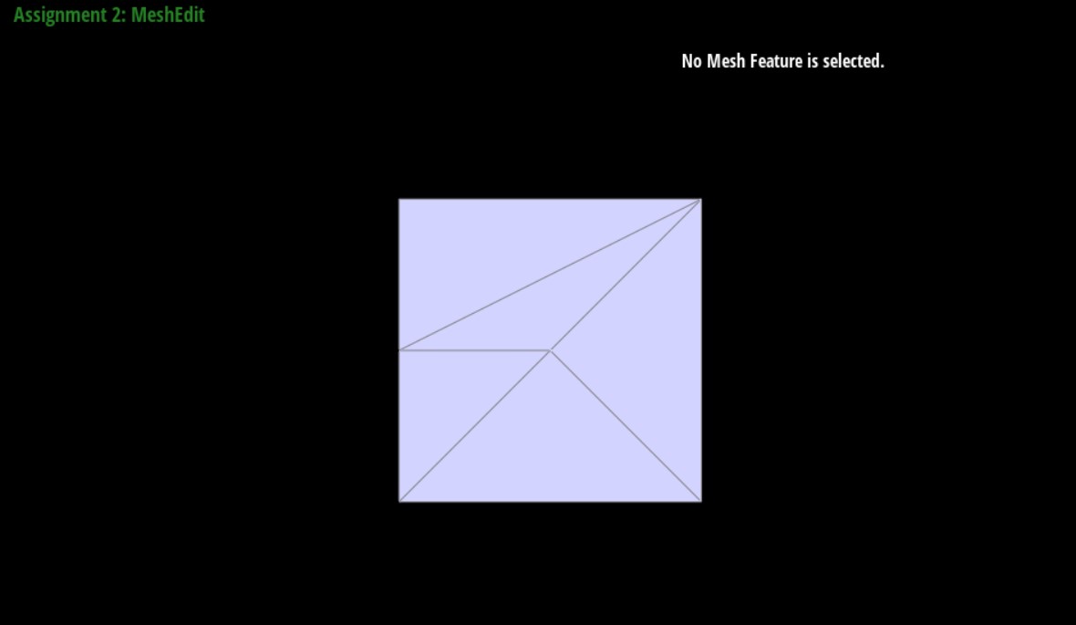
Original Image

After an Edge Split

After Many Edge Splits

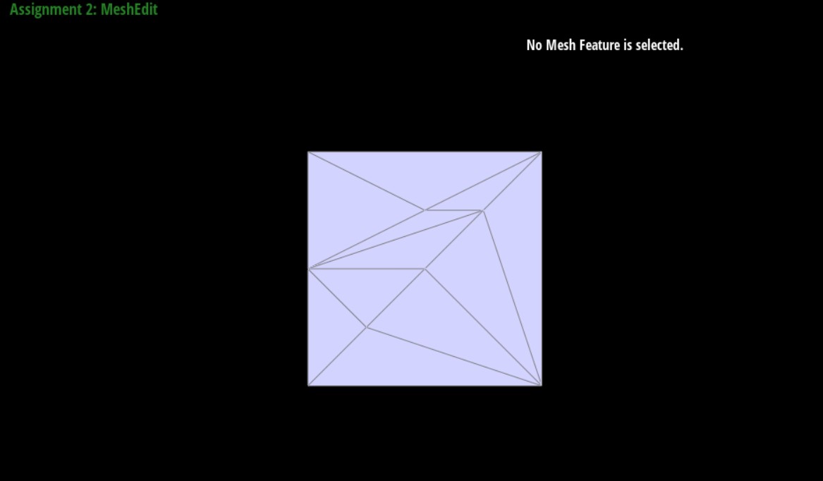
After Edge Splits and a Flip

Debugging Journey: Due to our detailed analysis when creating the diagram and table of changes required for an edge split, our diagram and table were correct by the time we implemented the function. The only bugs we ran into were ones caused by misassigning pointers, for example at first we accidently defined the split point position using the the two points not along the edge instead of the points along the edge.

Part 6: Loop Subdivision

Loop subdivision is an algorithm that allows for upsampling of 3D meshes by splitting edges, then computing new positions for vertices. The result of this algorithm is that a mesh becomes smaller and more rounded, approaching some eventual shape with no corners or sharp edges.

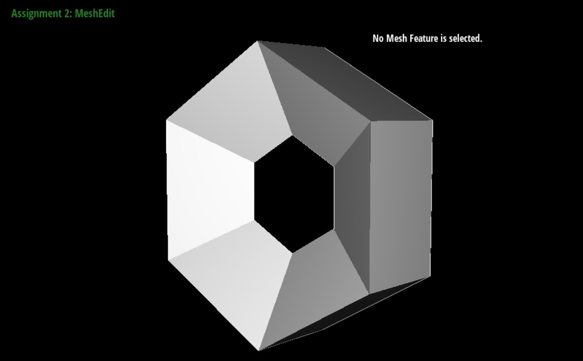
For example, here is a hexagonal torus with no Loop subdivision:

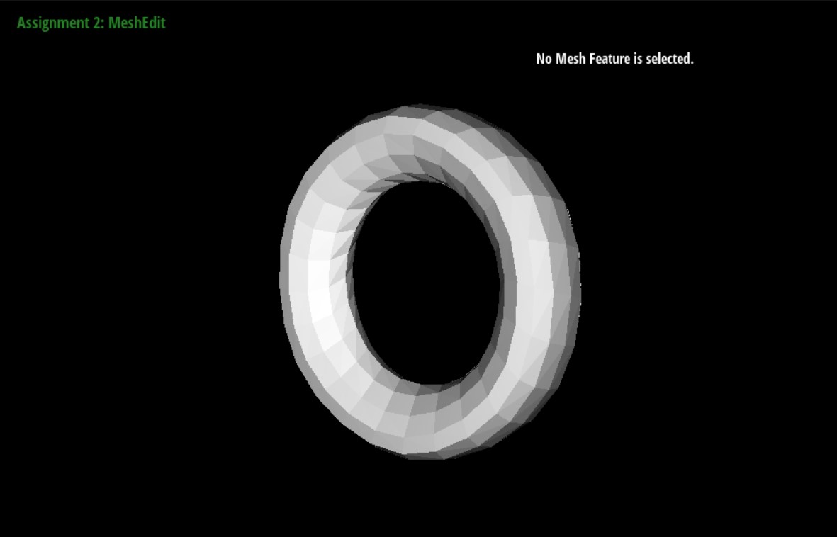
After subdividing it twice, we can see that it has become much more circular:

We implemented upscaling via Loop Subdivision using the suggested 5 steps:

Step 1:

Compute new positions for all vertices. We did this using the HalfedgeMesh::VertexIter class to iterate through every vertex.

The formula for doing so is as follows:

1. Iterate through each neighboring vertex using h->next()->vertex() until we reach the original halfedge h again. While doing so, save the count of vertices seen to n, and add each vertex position to neighbor_sum.
2. Initialize $u$ to $3/16$ if $n$ is $3$, and $3/(8n)$ otherwise.
3. Use the following formula to save the position to newPosition: v->newPosition = (1 - n * u) * v->position + u * neighbor_sum

In addition, we must set isNew to false for every vertex seen in this iteration.

Step 2: Compute the positions for all the new vertices. We used the HalfedgeMesh::EdgeIter class to iterate through every edge.

For each edge, we found the position of the new vertex that would be created along that edge using the following formula: $\frac{3}{8} (A + B) + \frac{1}{8} (C + D)$ where the edge is from A to B and C and D are the points associated with the two triangles on either side of the edge.

Step 3: Iterate through every edge, splitting each edge where isNew is false. The value isNew is set within splitEdge() for all of the edges newly created, to prevent infinite iteration.

Step 4: Flip any new edge that connects and old vertex to a new vertex. We itereated through all the edges and called flipEdge on the ones that satisfied the following conditions:

1. The edge had to connect an old vertex to a new vertex. We modified splitEdge to set the isNew field of the new vertex as true, and used that field to check that the given edge was between an old and new vertex.
2. The edge had to be a new edge. We used the edge’s isNew and isBlack fields to check that it was a new edge. isNew needed to be true since that indicated a new edge, isBlack needed to be false since that indicated an edge that the result of it being split (but would be considered an old edge by this algorithm)

Step 5: Update all of the vertex positions:

• For old vertices, their positions are stored in newPosition, so we can simply copy the value back to position.
• For new vertices, we instead iterate over the list of edges. If the edge is not new, it will have been split, so we can store its newPosition value into its corresponding new vertex at e->halfedge()->next()->vertex().

Several Steps of Loop Subdivision

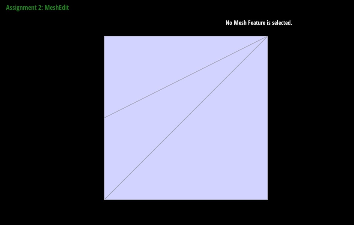
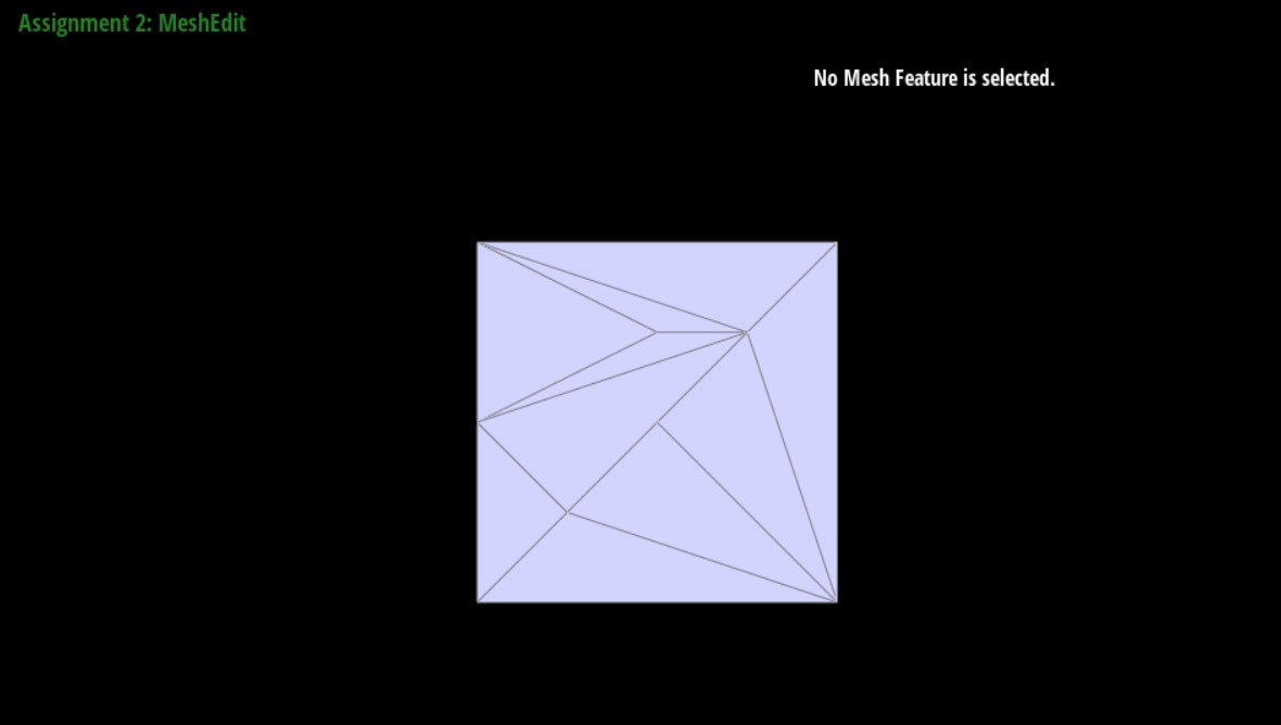
Starting from the standard cube.dae results in asymmetry, as seen below:

After one subdivision:

After two subdivisions:

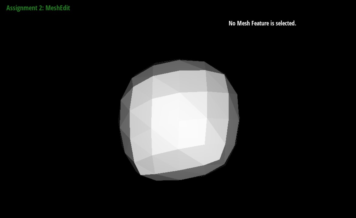
After three subdivisions:

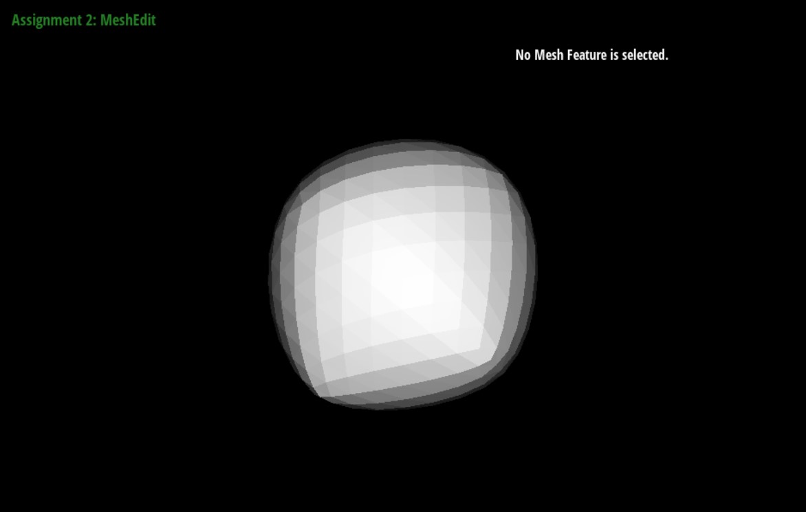
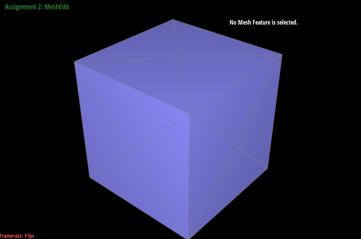
To resolve this issue, we can preprocess the cube by splitting every edge in the middle of a face. The asymmetry was created by the fact that the face had a diagonal only in one direction, so Loop subdivision would make that axis longer.

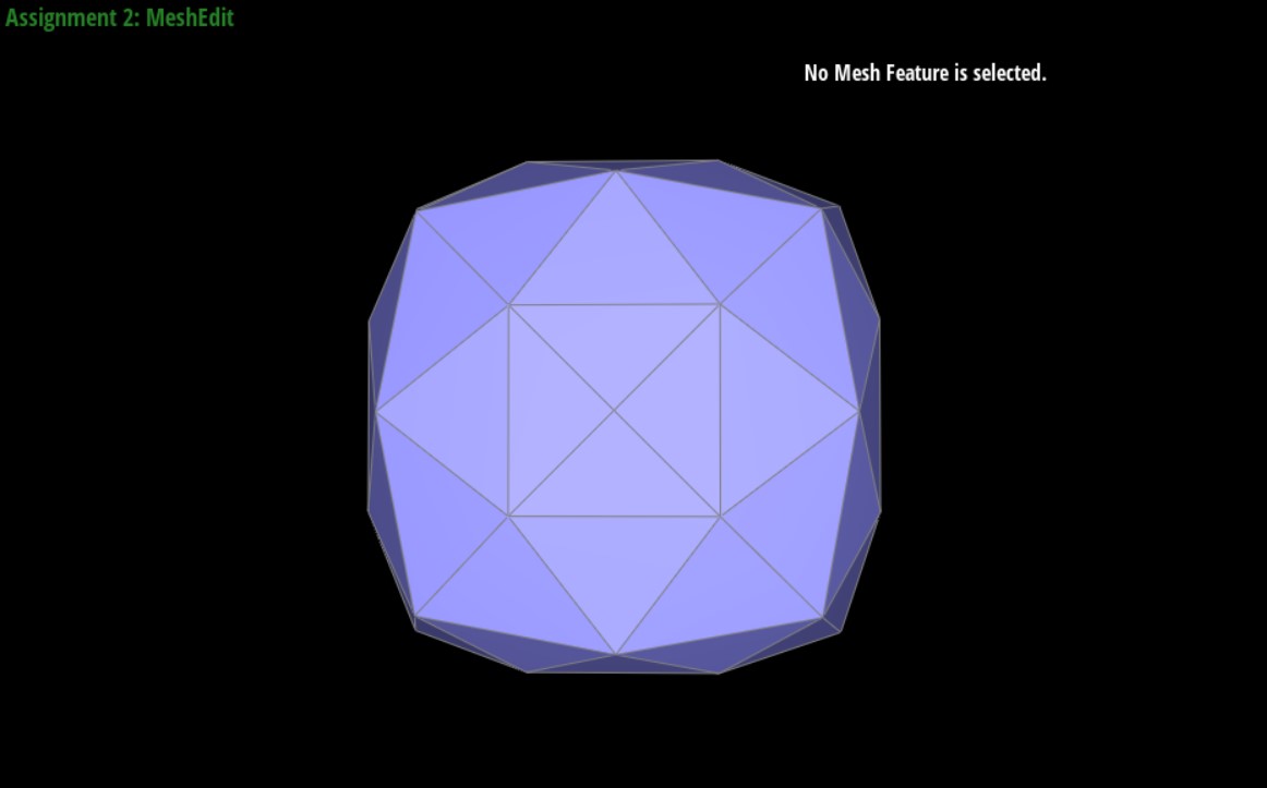
The preprocessed cube looks like this:

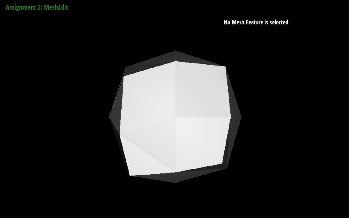
After one subdivision:

After many subdivisions: